Evaluating detection
Detecting AI-Generated Images: Accuracy and False Positives
Understand accuracy, false positives and score limits in detection of AI-generated images. Use a worked evaluation to compare thresholds, review workload and uncertainty.
Published · 12 min read
On this page
AI image detector accuracy is useful only when you know the task, the images tested and the rule used to turn scores into decisions. A detector can classify almost every image correctly while sending more false alarms than true detections to a review queue. A small queue can also conceal substantial numbers of missed images.
To evaluate a detector, ask three connected questions: what does it detect, what errors occur at the intended threshold, and what happens to files it cannot assess? The worked examples below connect those answers to the review work your team will receive.
For a quick check of an accuracy claim, start with the confusion matrix, prevalence and threshold sections. They show why a high accuracy figure can coexist with a poor review queue. If you own an evaluation, continue through calibration, coverage and the holdout design, then use the evidence request at the end. All numerical examples are hypothetical, not Fileverity results or fraud-prevalence estimates.
Define what counts as a positive
Begin with a sentence such as: “This evaluation tests whether an entire submitted image was AI-generated.” That definition makes fully generated images positive cases and qualifying camera photographs negative cases. It does not establish a test for localized AI edits, conventional retouching, misleading captions or recycled photographs.
If your workflow requires detection of partial generation, evaluate that as a separate task with explicit labels. A camera photograph containing a generated region should not silently move between the positive and negative groups depending on which interpretation improves a result. Likewise, permitted AI use is not necessarily deceptive. Detection labels describe content; policy and corroborating evidence determine its significance.
Define the unit, too. Five images from one submission are five image decisions but perhaps only one investigation. Image-level accuracy will not directly predict case-level review workload when one flagged image triggers a review of the whole submission.
Read the confusion matrix before the headline
A confusion matrix compares detector decisions with independently established labels. Consider 10,000 hypothetical images: 100 generated images and 9,900 non-generated images. At one fixed threshold, the detector flags 90 generated images and 99 non-generated images.
| Known label | Flagged | Not flagged | Total |
|---|---|---|---|
| Generated | 90 true positives (TP) | 10 false negatives (FN) | 100 |
| Not generated | 99 false positives (FP) | 9,801 true negatives (TN) | 9,900 |
| Total | 189 | 9,811 | 10,000 |
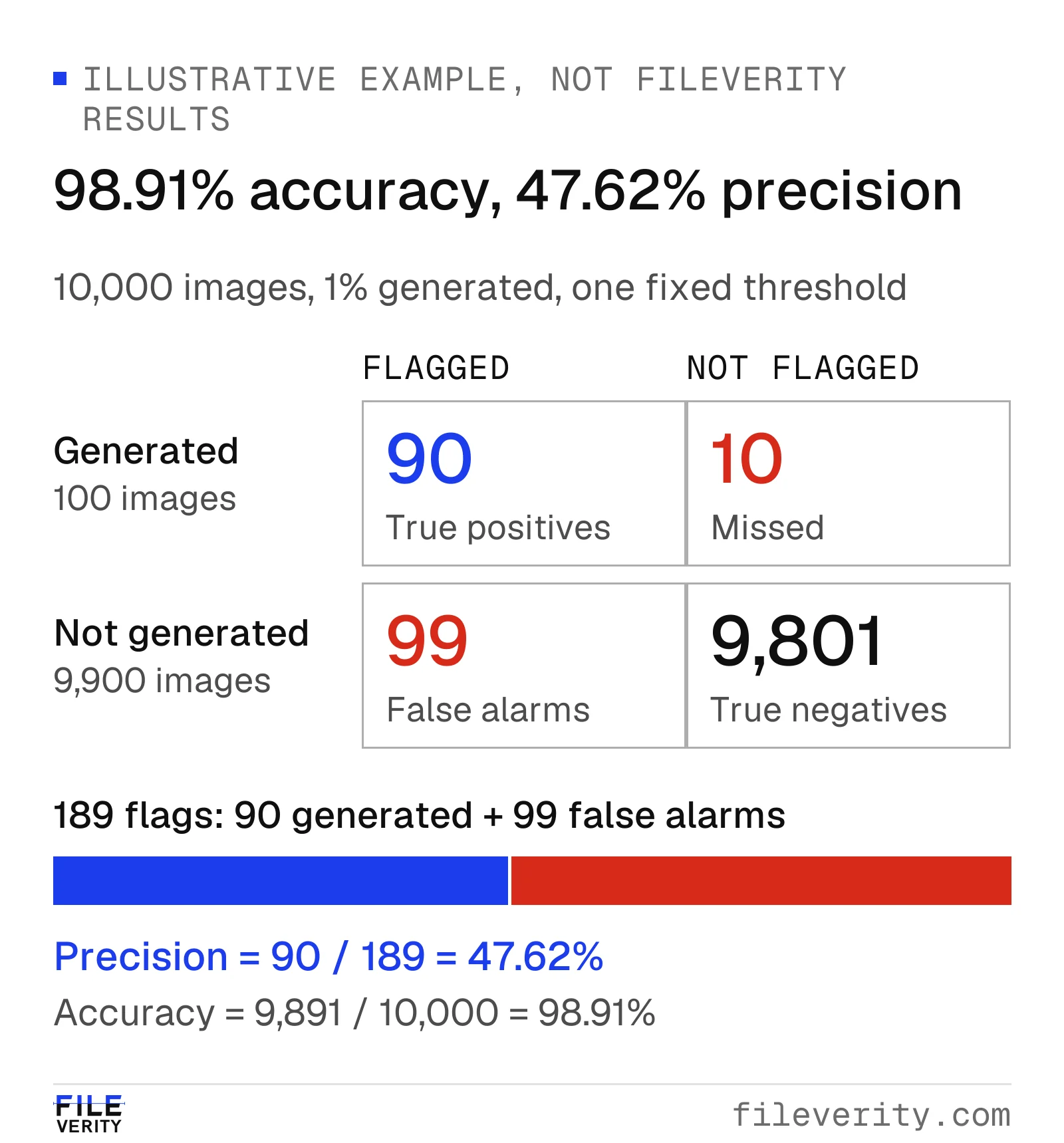
Of 189 flags, 90 are correct and 99 are false alarms—even though overall accuracy is 98.91%.
Each metric answers a different question:
| Metric | Calculation | Result | Question answered |
|---|---|---|---|
| Accuracy | (TP + TN) / all images | 98.91% | How many decisions were correct? |
| Recall, or sensitivity | TP / (TP + FN) | 90% | How many generated images were found? |
| False-negative rate | FN / (TP + FN) | 10% | How many generated images were missed? |
| False-positive rate | FP / (FP + TN) | 1% | How many non-generated images were flagged? |
| Specificity | TN / (FP + TN) | 99% | How many non-generated images avoided a flag? |
| Precision, or positive predictive value (PPV) | TP / (TP + FP) | 47.62% | How many flags were correct? |
Precision is rounded from 90/189. The distinction between false-positive rate and precision is crucial: a 1% false-positive rate does not mean that only 1% of the flagged images are false alarms. The denominators differ. Here, 99/189, or 52.38%, of flags are false alarms. Standard definitions and their relationship to confusion matrices are documented in scikit-learn's classification metrics reference.
An always-negative rule would achieve 99% accuracy on this same collection while finding none of the generated images. That does not make it a useful detector. It shows why a headline accuracy comparison can reward the wrong behavior when one class dominates.
Calculate what prevalence does to the queue
Prevalence is the proportion of positive cases in the population being evaluated. In this example it is 1%. When recall and false-positive rate are held fixed, expected precision follows this relationship:
PPV = (recall × prevalence) / [(recall × prevalence) + (false-positive rate × (1 − prevalence))]
Using proportions, the calculation is 0.90 × 0.01 / [(0.90 × 0.01) + (0.01 × 0.99)] = 0.009/0.0189 = 47.619…%.
The scenarios below use expected counts, so a fractional count describes an average expectation rather than an observed fraction of an image.
Hypothetical expected outcomes per 10,000 images, holding recall at 90% and false-positive rate at 1%.
| Hypothetical prevalence | Expected true flags | Expected false flags | Expected precision |
|---|---|---|---|
| 0.1% | 9 | 99.9 | 8.26% |
| 1% | 90 | 99 | 47.62% |
| 10% | 900 | 90 | 90.91% |
| 50% | 4,500 | 50 | 98.90% |
A balanced benchmark can therefore produce impressive precision that does not transfer to a low-prevalence intake. This calculation assumes the class-specific performance stays unchanged. In practice, a different intake may also contain harder images, changing recall and false-positive rate themselves.
Do not estimate prevalence from the fraction flagged: that fraction includes errors. Use an independently labeled sample of the intake, report unresolved labels, and test several plausible prevalence scenarios if the estimate remains uncertain. Use those scenarios to budget review capacity before committing to a threshold.
Choose a threshold for the action it triggers
For a score where larger values indicate stronger evidence of generation, lowering the flag threshold includes more images. On the same scored dataset it cannot remove previously flagged images, so it can increase both true detections and false alarms. Raising it reverses that direction. Precision need not improve at every threshold step; the ordering of actual labels determines that.
Here is a constructed comparison on the same 10,000-image population. No real score cutoffs are assigned because score scales differ between systems.
Hypothetical threshold comparison: the same 100 generated and 9,900 non-generated images at each threshold.
| Threshold | True positives | False positives | Missed positives | Recall | False-positive rate | Precision | Queue size |
|---|---|---|---|---|---|---|---|
| Lower | 95 | 297 | 5 | 95% | 3% | 24.23% | 392 |
| Middle | 90 | 99 | 10 | 90% | 1% | 47.62% | 189 |
| Higher | 70 | 20 | 30 | 70% | 0.202% | 77.78% | 90 |
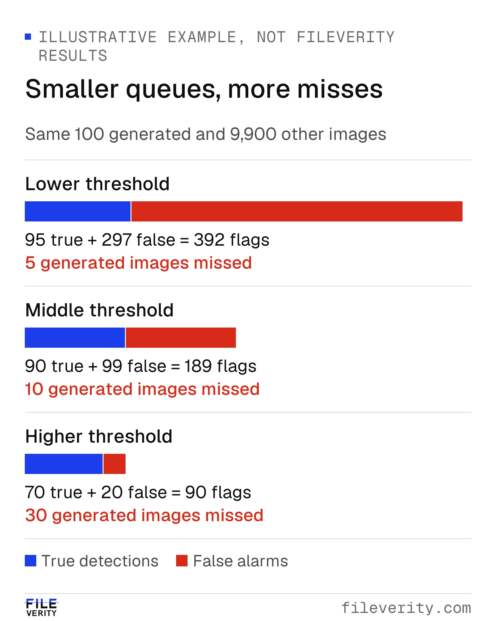
Raising the threshold reduces the review queue from 392 to 90 images, while increasing missed positives from 5 to 30.
At a hypothetical six minutes per flagged image, these queues require 39.2, 18.9 and 9 staff-hours respectively, before additional investigation. Choosing the smallest queue also accepts 30 misses instead of five. Neither choice is inherently correct: the intended action, available reviewers and consequences of errors determine what is acceptable.
Request performance at the operating point you intend to use. An ROC curve summarizes recall against false-positive rate across thresholds; its area does not tell you the recall at your particular false-alarm limit. NIST specifically discusses reporting true-positive rate at a specified low false-positive rate when false accusations carry substantial consequences. NIST AI 100-4, section 4.2.2 and Appendix E
Distinguish confidence from calibration
A score of 90 could be a ranking signal, a transformed model output or a probability estimate. It is not automatically a 90% probability of generation, and it does not mean that 90% of the pixels were edited. Obtain the score definition before attaching meaning to the number.
Calibration asks whether probability estimates agree with observed frequencies across comparable cases. Discrimination asks whether the scores separate the target categories. Both matter, but neither substitutes for the other. The worked diagnostic below shows how to examine the probability claim before using it in an operating policy.
Inside the score: test calibration with observed frequencies
Calibration is the property to test in any detector, including ours. The table below is an illustrative evaluation, not Fileverity data. A concrete way to inspect calibration is a reliability diagram: group predictions into probability ranges, then compare each group's average prediction with its observed positive frequency.
For a group B, calculate p̄_B = Σp_i/n_B and r_B = Σy_i/n_B, where p_i is the predicted probability, y_i is 1 for an independently established positive and 0 otherwise, and n_B is the group size. Perfect agreement in that group means p̄_B = r_B. It does not mean each individual prediction is certain. Guo and colleagues discuss reliability diagrams and calibration measurements in neural classification. Guo et al., ICML 2017
Consider this illustrative binary generation evaluation:
| Probability range | Images | Average prediction | Known positives | Observed positive frequency | Absolute gap |
|---|---|---|---|---|---|
| 0.0–<0.4 | 100 | 0.20 | 10 | 0.10 | 0.10 |
| 0.4–<0.7 | 100 | 0.50 | 40 | 0.40 | 0.10 |
| 0.7–1.0 | 100 | 0.80 | 60 | 0.60 | 0.20 |
A sample-weighted absolute bin gap is Σ(n_B/N) × |p̄_B − r_B|. Here it is (0.10 + 0.10 + 0.20)/3 = 0.1333, or about 13.3 percentage points. This describes disagreement in these groups; it is neither a classification error rate nor a claim that every score is wrong by 13.3 points. Different bins can hide or reveal different discrepancies, so retain the counts and diagram alongside the summary.
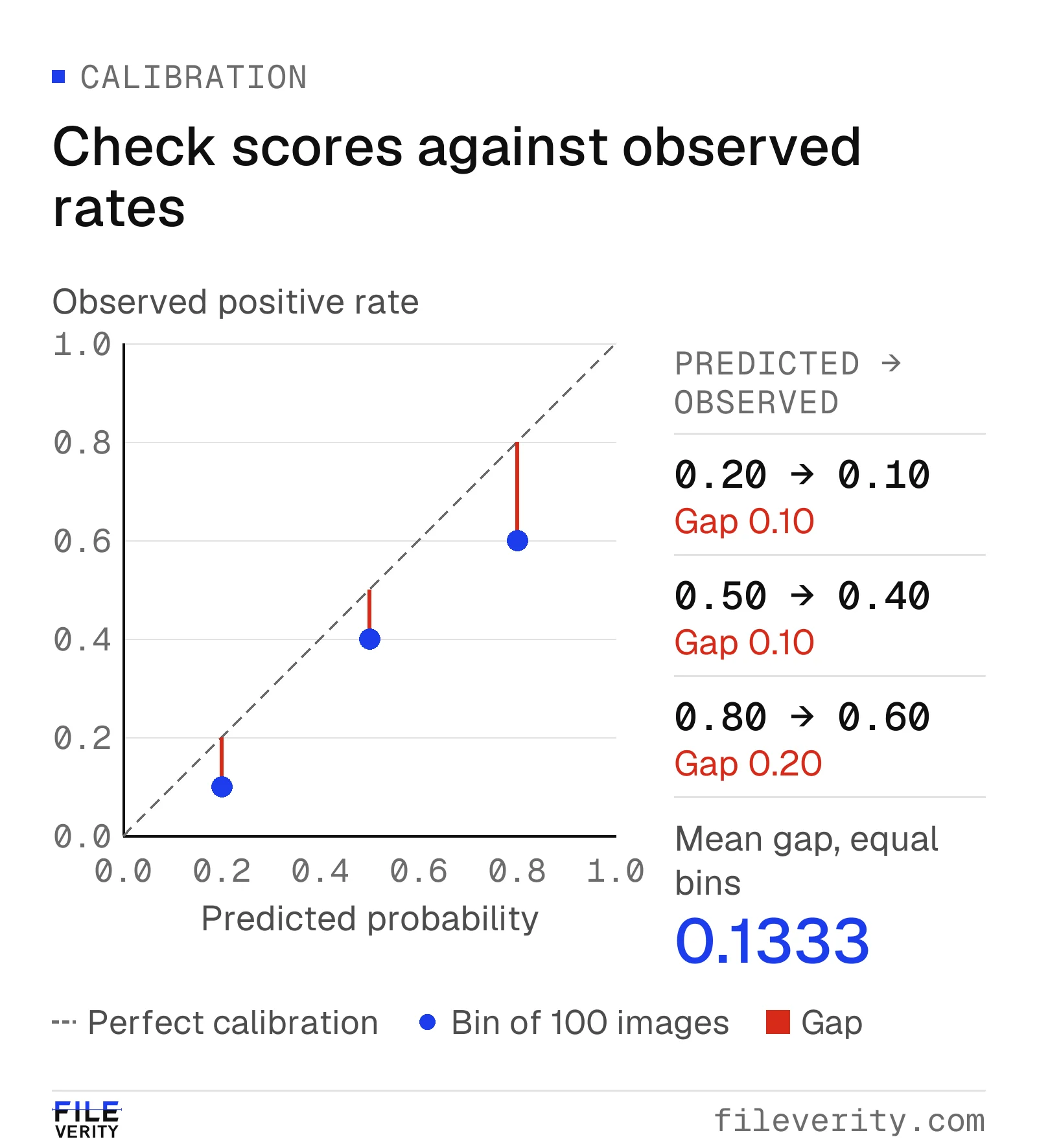
Illustrative calibration data, 100 images per group: predictions exceed observed positive frequencies by 10, 10 and 20 percentage points.
Why can calibration improve without better discrimination? A strictly increasing score transformation preserves every pair's order, so a ranking metric such as ROC AUC remains unchanged, while probability values can move closer to observed frequencies. The numerical cutoff associated with the same decisions can change. Consequently, ask for evidence about both ranking or operating-point errors and probability interpretation.
Calibration also depends on the evaluated population. Ovadia and colleagues show that uncertainty estimates can deteriorate under dataset shift. Ovadia et al., NeurIPS 2019 Fit any mapping separately from the final acceptance sample; then inspect relevant submission channels individually. Include your own intake channels in that calibration check.
Keep uncertain and unsupported files in the denominator
A detector may abstain, reject an unsupported format, time out or return a low-quality warning. These outcomes need separate counts. Excluding them can make a system appear reliable precisely because its hardest cases disappeared.
Consider another hypothetical batch: 1,000 submissions, of which 850 receive a usable classification, 100 receive an uncertain result and 50 fail processing. Classification coverage is 850/1,000 = 85%. If 833 classifications are correct, accuracy among classified files is 833/850 = 98%. Across all submissions, 83.3% received a correct classification; this is a coverage-aware descriptive figure, not conventional binary accuracy. The other 150 are unresolved, not automatically incorrect or negative.
Report accuracy and coverage together, then break coverage down by known label and intake channel. A system may abstain more often on positive cases. Report overall recall with an explicit treatment of abstentions, alongside recall restricted to classified cases, so users can see what each denominator excludes. Provide a fallback route for unresolved files and include that route in workload estimates.
Build a representative, untouched holdout
An evaluation needs defensible labels and a sampling plan. Use authorized material with documented origins: controlled generated examples, camera originals with known capture histories, and separately labeled edits where relevant. Another detector's opinion is not ground truth. Retain disputed labels as unresolved and document the adjudication rule.
Match the received files, not merely pristine originals. Include the channels, image sizes, content categories and ordinary handling histories your workflow encounters. Keep related variants of a source image together when splitting data; otherwise the same underlying scene can leak into both tuning and evaluation. Where possible, also separate capture sessions and source collections.
Use a development set to choose thresholds and a distinct holdout to check the chosen policy once. If a failed holdout prompts changes, treat it as development evidence and obtain a new untouched test for the revised policy. For proprietary services, ask about known overlap with public benchmarks and acknowledge what training-data overlap cannot be checked.
Keep a deliberately difficult challenge set as a supplement. Report it separately from the representative sample so that oversampling unusual cases does not masquerade as normal intake prevalence. Research on generated-image detection tests generalization across generators precisely because success on one source does not establish universal coverage. Wang and colleagues, CNN-generated images are surprisingly easy to spot… for now
Set acceptance criteria before looking at results
Write an evaluation record that connects each metric to the decision it must support.
Example acceptance criteria for a workflow that routes images to human review.
| Item | Example criterion or record |
|---|---|
| Intended use | Route images for human review; no automatic adverse decision |
| Frozen configuration | Service version, threshold, score definition and preprocessing recorded |
| False alarms | One-sided 95% upper confidence bound for FPR no greater than 1% |
| Detection | One-sided 95% lower confidence bound for recall at least 85% |
| Coverage | At least 95% classified; every unresolved file has a fallback route |
| Capacity | Total review and fallback workload fits a preassigned daily staffing budget |
| Subgroups | Report critical intake channels separately; insufficient evidence remains unresolved |
| Decision owner | Named reviewer records acceptance, rejection or a limited pilot |
Confidence bounds prevent a small clean sample from being mistaken for certainty. With zero false positives among 300 independent negative cases, the exact one-sided 95% binomial upper bound is 1 − 0.05^(1/300), approximately 0.994%. With zero among 100, it is approximately 2.951%.
The derivation is short: if the false-positive probability is p, the probability of zero false positives in n independent negative cases is (1 − p)^n; setting this to 0.05 gives the upper bound p = 1 − 0.05^(1/n). Zero observed errors therefore does not establish a zero error rate. These calculations assume independent, representative cases; many near-duplicate photographs do not supply the same evidence as independent submissions.
The middle-threshold example's observed 1% false-positive rate would not pass a requirement that its upper confidence bound be at most 1%. A point estimate and an uncertainty bound answer different questions. Plan the sample size around the required evidence before collecting the test set.
Monitor drift and phrase conclusions carefully
After deployment, monitor flag rates, unresolved rates, channel mix, review time and independently confirmed outcomes. A rising flag rate alone cannot distinguish more generated images from increased false alarms. Sample unflagged cases as well; reviewing only flags leaves missed positives largely invisible. Account for sampling probabilities when estimating intake-wide metrics from deliberately oversampled groups.
Record changes to the model, threshold and intake process. Re-evaluate after a material change, and maintain periodic labeled checks even when dashboard averages appear stable. A new generator, submission channel or content category may change performance without an obvious overall alert.
Separate the observation from the decision in a case record: “The image exceeded the review threshold” is an observation. “This supports a concern about generation” is an inference. A verified original or documented creation history provides corroboration. Requesting that material is an action. None of these statements alone establishes fraud or the truth of the scene depicted.
Turn an accuracy claim into an evidence request
Ask for enough information to connect the claimed result to your intake and your next action. You can copy the following request into a vendor discussion:
We need to assess [whole-image generation / local alteration / another defined task] on [file formats, channels and quality conditions]. The result will trigger [review action], at approximately [daily images and cases]. Our review capacity is [staff-hours or cases per day].
Please provide the evaluated product version and score definition; label sources and positive/negative counts; all four confusion-matrix counts at the proposed operating point; uncertainty estimates; and separate counts for inconclusive, unsupported and failed inputs. State which files are excluded from each metric, how coverage and recall change when those files are included, and whether related source images overlap across tuning and evaluation.
Identify which evidence applies to this use, which conditions remain untested, and what a pilot would need to establish.
Fileverity reports each result by task, shows inconclusive and unsupported inputs as separate outcomes instead of hiding them, and states the strength of the evidence behind each finding; how the image analysis works is set out on the image analysis method page. Send us your evidence request and your intake channels, and we will walk your team through it on real cases; talk to sales. For the wider purchase decision, including data handling and total review cost, continue with the AI image detection software buyer's checklist.
By Yang Zheng · Reviewed by Bill Liu